
TL;DR
- OpenObserve's benchmark of one billion Kubernetes log records has it finishing the query set several times faster than ClickHouse, with one query at 109x, on about a third less disk.
- The ClickHouse table is ordered by
_timestampalone and relies on Bloom filters, while OpenObserve uses Tantivy indexes. The largest gaps reflect those index and physical design choices, not DataFusion against the ClickHouse execution engine. - Four of the 19 queries account for most of the gap. With those removed, the totals in the table below are 3.0 s for ClickHouse against 3.3 s for Parquet and 2.8 s for Vortex.
- The benchmark excludes projections and materialized views, yet OpenObserve answers the hourly histogram from metadata produced ahead of time, so that comparison is asymmetric.
- A fairer follow-up keeps the current ClickHouse table as a baseline and adds one designed for the workload, then repeats the queries over several time windows.
OpenObserve recently published a benchmark comparing OpenObserve with ClickHouse using one billion Kubernetes log records. At initial glance, the numbers are pretty rough for ClickHouse, but I guess as a product vendor the blog has to favour its own product, I get it. OpenObserve finishes the complete query set several times faster, one query is reported as more than 100x faster, and the Parquet data takes substantially less disk.
I went through the schema and queries because the storage figure surprised me. Parquet and ClickHouse are both columnar, both compress repeated values well, and ClickHouse is normally very good at this sort of workload. The public benchmark repository makes it possible to see where the large differences come from rather than trying to infer them from the final timings.
The 109x result comes from the sorting key, not the query engine
The ClickHouse sorting key is a good place to start.
ENGINE = MergeTree
ORDER BY (_timestamp)
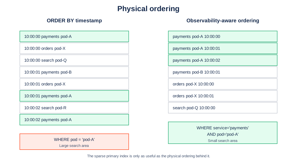
That choice has a large effect on ClickHouse because rows are physically arranged by the sorting key and the sparse primary index follows that layout. With timestamp as the only key, records from different pods, namespaces, services and containers are mixed together throughout each part.
With timestamp as the only sorting key, the rows end up interleaved in a pattern like the one below.
10:00:00  payments  pod-A
10:00:00  orders    pod-X
10:00:00  search    pod-Q
10:00:01  payments  pod-B
10:00:01  orders    pod-X
10:00:01  payments  pod-A
10:00:02  search    pod-R
10:00:02  payments  pod-A
A query for one pod then has to work against that physical layout.
WHERE kubernetes_pod_name = 'pod-A'The ClickHouse primary index has very little to work with because kubernetes_pod_name is not in the sorting key. The benchmark adds a Bloom filter, which can rule out granules that definitely do not contain the pod name, but a Bloom filter does not tell ClickHouse which rows match.
OpenObserve uses Tantivy for the corresponding secondary index, so it can keep a posting list that maps a pod name much more directly to the matching documents.
pod-A → row 12, row 91, row 430, row 1229, ...The 109x pod-name result is much easier to understand once those two access paths are put side by side. OpenObserve can go from the pod name to matching documents through Tantivy. The benchmarked ClickHouse table has timestamp ordering and a Bloom filter, so it has to inspect far more of the table. This is not a 109x difference between DataFusion and the ClickHouse execution engine.
OpenObserve says in the article that a ClickHouse engineer would probably change the sorting key and add column codecs. They also note that a pod-oriented key would change the pod-name result substantially. That caveat deserves to sit next to the 109x number because the result depends heavily on the physical design chosen for the ClickHouse table.
A ClickHouse schema built for log queries
I would not start a large Kubernetes or OpenTelemetry log store with ORDER BY (_timestamp) unless time was genuinely the only access pattern I cared about. The exact key should come from the workload, but a more deliberate table could look like this.
CREATE TABLE logs
(
    timestamp_ns Int64
        CODEC(DoubleDelta, ZSTD(1)),

    service LowCardinality(String),
    namespace LowCardinality(String),
    pod LowCardinality(String),
    container LowCardinality(String),

    severity UInt8,

    trace_id FixedString(16),
    span_id  FixedString(8),

    body String CODEC(ZSTD(1)),

    INDEX body_text body
        TYPE text(tokenizer = splitByNonAlpha)
)
ENGINE = MergeTree
PARTITION BY toDate(fromUnixTimestamp64Nano(timestamp_ns))
ORDER BY
(
    service,
    namespace,
    pod,
    timestamp_ns
);
There is no universal sorting key for logs, and this example is only meant to show how much of ClickHouse's physical design is absent from the benchmark configuration.
Types and codecs are another part of the physical design that changes the result. Fields such as service, namespace and container repeat constantly and are obvious candidates for LowCardinality(String). Trace and span IDs can use fixed-width representations instead of generic strings. Timestamps are a good fit for DoubleDelta, and ClickHouse also provides Delta, Gorilla and T64 for other data patterns.
The storage figures need to be read with that in mind. The benchmark reports roughly 1,026 GB for ClickHouse and 674 GB for OpenObserve using Parquet. Both systems are columnar and both can compress repeated data aggressively. The result shows that OpenObserve's representation, encoding and indexes are smaller than the ClickHouse configuration used in the benchmark. It does not tell us that Parquet is inherently about a third smaller than MergeTree.
One table does not mean one access path
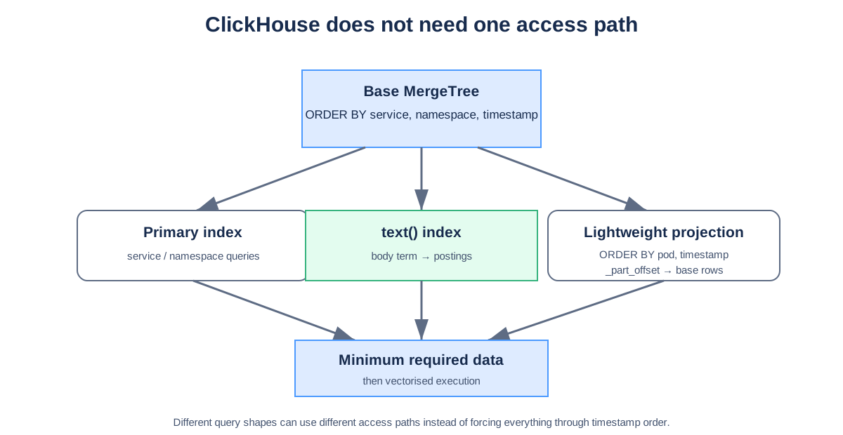
No single sorting key can suit every query, but ClickHouse has other ways to add access paths. Projections can maintain another ordering, and lightweight projections can point back into the base part through _part_offset rather than duplicating every column.
A logging system could therefore keep a base ordering aimed at service and namespace queries, another path for pod lookups, and a text index for message search. That is a very different ClickHouse design from a timestamp-ordered table backed by Bloom filters.
The hourly histogram uses different work on each side
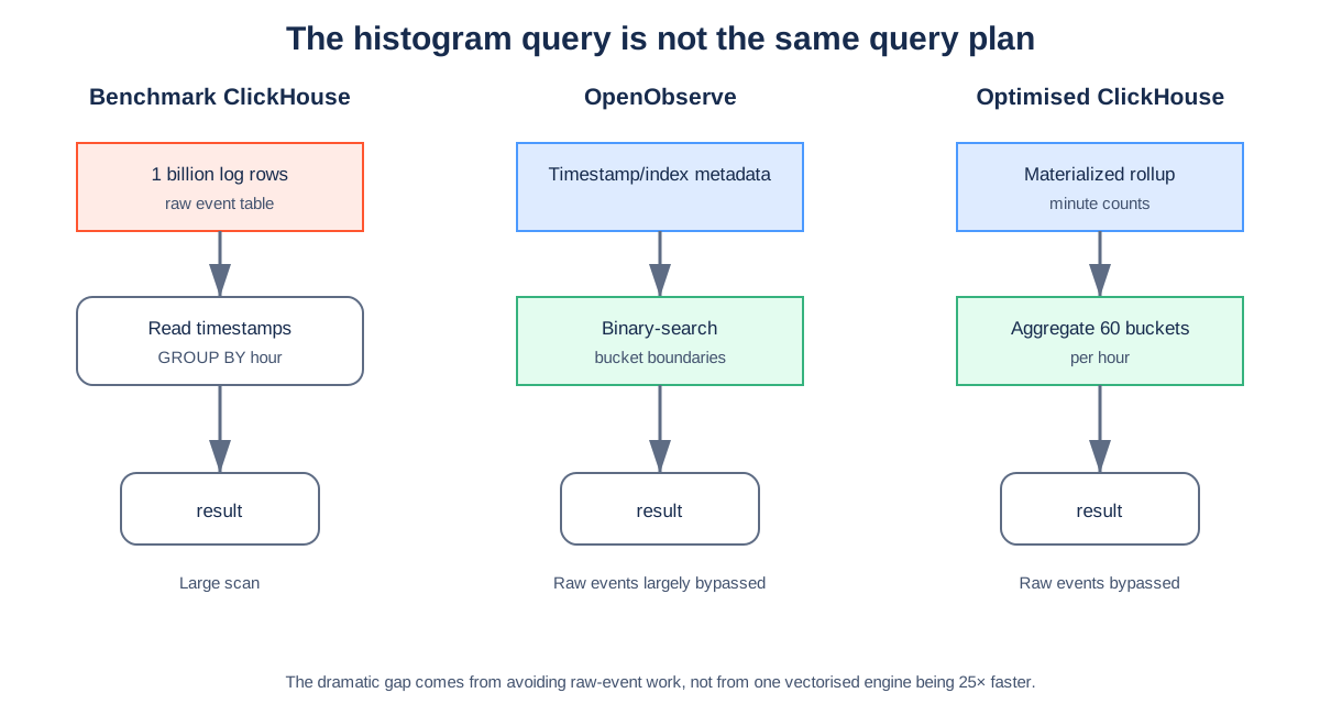
The hourly histogram is one of OpenObserve's largest wins. OpenObserve answers it in tens of milliseconds while ClickHouse takes around 1.6 seconds. The explanation in the OpenObserve article is more revealing than the timing itself because OpenObserve can use timestamp information held with its index files to calculate bucket counts without processing all one billion timestamps in the normal way.
The ClickHouse query in the benchmark reads timestamps from the raw data and aggregates them. The two systems are therefore executing different amounts of work.
ClickHouse benchmark
    raw logs → timestamps → GROUP BY hour

OpenObserve
    index metadata → bucket boundaries → result
If I were building the same dashboard capability on ClickHouse, I would not recalculate those counts from the raw table every time. I would populate a small aggregate table during ingestion and query that instead.
CREATE TABLE log_counts_1m
(
    bucket      DateTime,
    fingerprint UInt128,
    count       SimpleAggregateFunction(sum, UInt64)
)
ENGINE = AggregatingMergeTree
ORDER BY (fingerprint, bucket);
An hourly chart can aggregate minute-level counts from this table and leave the billion raw log records alone. OpenObserve has chosen a different implementation, but both approaches remove most of the raw-data work from the query.
The benchmark excludes materialized views and projections because they are treated as precomputed answers, which makes this particular comparison asymmetric. OpenObserve can use metadata produced ahead of time to skip the raw events, while the ClickHouse side is prevented from using common ClickHouse mechanisms that an observability product could use for the same purpose.
Four queries account for most of the gap
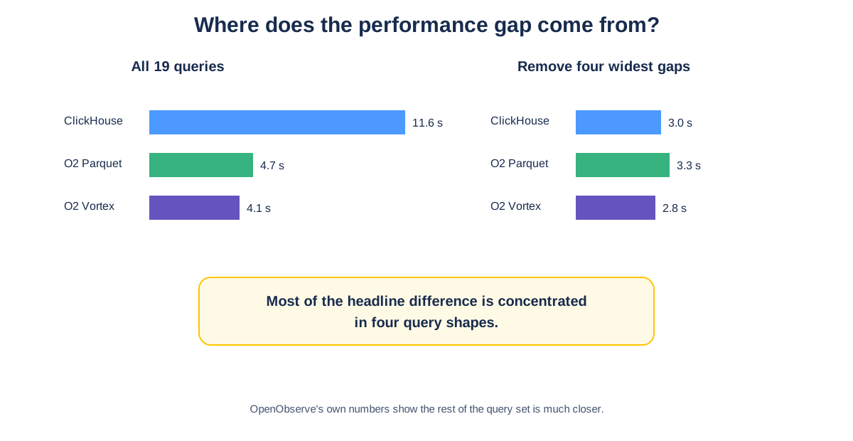
OpenObserve also publishes the totals after removing the four queries with the largest differences.
| Query set | ClickHouse | OpenObserve Parquet | OpenObserve Vortex |
|---|---|---|---|
| All 19 queries | 11.6 s | 4.7 s | 4.1 s |
| Without the four widest gaps | 3.0 s | 3.3 s | 2.8 s |
Across the remaining fifteen queries, ClickHouse and Parquet are essentially level and Vortex is a little quicker. Most of the total difference comes from a small set of queries where OpenObserve has an index or metadata path that the benchmarked ClickHouse table does not have.
That tells us quite a lot about the indexing strategy. It tells us much less about the relative speed of DataFusion and ClickHouse when both engines process comparable amounts of columnar data.
The text searches are much closer
The full-text results provide a useful comparison because both systems have an inverted index available. The rare-token query is roughly tied, and ClickHouse is quicker on the two-token intersection in the published numbers.
Once both systems can turn a search into posting lists, neither side needs to scan one billion message strings.
"connection" AND "timeout"The query becomes an intersection of postings, so the result depends much more on the index implementation than on whether the underlying data sits in Parquet or MergeTree.
OpenObserve has an advantage on some common-token count queries because Tantivy can derive the count cheaply from its postings. I would keep that query in any follow-up benchmark because it tests a capability that the ClickHouse text index may not answer in the same way.
The one-year window removes normal time pruning
The billion records span roughly four hours and thirteen minutes, while the benchmark queries use a one-year window that keeps the complete data set eligible. OpenObserve explains that this was done so neither system benefits from partition pruning.
That is a reasonable worst-case test, but operational log searches usually begin with a much smaller time range. An incident investigation will often start with the last 15 minutes or the last hour and grow only if the operator needs more history.
I would keep the full-retention query and then repeat the same workload over 15 minutes, one hour, six hours and one day. That shows how the systems behave under the access patterns people use during an incident as well as under a deliberately broad scan.
A log platform does not need a single flat event table
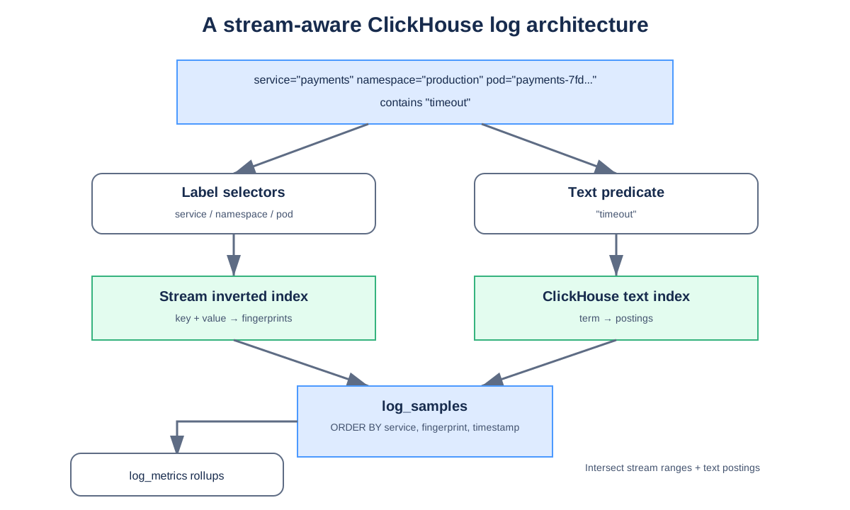
There is a bigger design question once the comparison moves from generic databases to observability products. OpenTelemetry and LogQL already give us the idea of a stable label set describing a log stream. The individual records mostly add time, severity and message content.
A ClickHouse-backed system can separate that stream identity from the samples rather than carrying all of the stable metadata through the large event population.
CREATE TABLE log_samples
(
    service       LowCardinality(String),
    fingerprint   UInt128,
    timestamp_ns  Int64 CODEC(DoubleDelta, ZSTD(1)),
    severity      Int8,
    body          String CODEC(ZSTD(1)),

    INDEX body_text body
        TYPE text(tokenizer = splitByNonAlpha)
)
ENGINE = MergeTree
PARTITION BY toDate(fromUnixTimestamp64Nano(timestamp_ns))
ORDER BY (service, fingerprint, timestamp_ns);
The stream labels can live in a much smaller index.
CREATE TABLE log_streams_idx
(
    key          LowCardinality(String),
    val          String,
    fingerprint  UInt128
)
ENGINE = ReplacingMergeTree
ORDER BY (key, val, fingerprint);
The benefit of separating stream identity becomes clearer with a normal LogQL-style query.
{service="payments", namespace="prod", pod="payments-7fd..."}
|= "timeout"
The label match can be resolved to stream fingerprints before the large samples table is touched. The sample lookup then uses service, fingerprint and time, which matches the physical ordering, and the text index only has to operate on the relevant sample population.
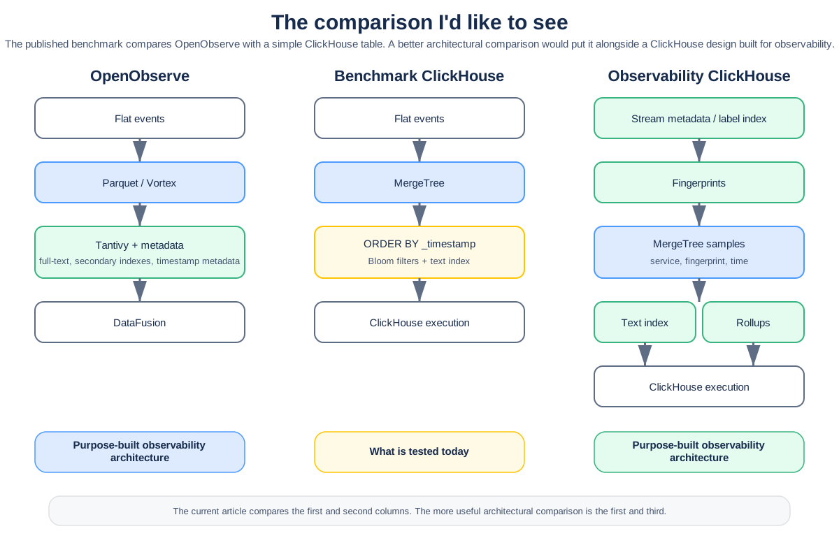
At that point both sides of the comparison are observability systems making workload-specific choices. That is a better test of OpenObserve against a ClickHouse-based logging architecture than comparing OpenObserve with a single generic wide table.
The follow-up benchmark I would run
I would keep the current ClickHouse configuration as a baseline, add a second one designed for the workload, and leave the OpenObserve configuration unchanged.
The second ClickHouse setup should be allowed to use a sorting key based on the query patterns, LowCardinality and fixed-width types where appropriate, telemetry-specific codecs, the ClickHouse text index, lightweight projections, and aggregate tables or materialized views for the query classes where OpenObserve also avoids reading raw events.
I would also repeat the queries across several time windows and collect more than elapsed time. Rows and marks read, compressed bytes read, S3 bytes fetched, CPU time, peak memory, index size, and cold-cache versus warm-cache behaviour would make the cause of each result much easier to see.
What the published numbers support
The benchmark is reproducible enough to inspect, which is why the large differences can be traced back to the schema, indexes and query plans. The measurements describe those two configurations rather than establishing that OpenObserve is generally three or four times faster than ClickHouse or that Parquet is inherently a third smaller than MergeTree.
OpenObserve gets its largest wins when it can avoid reading the whole event population through Tantivy or metadata created during ingestion. ClickHouse provides the pieces to build similar shortcuts through physical ordering, sparse indexes, text indexes, projections, materialized views, aggregate tables, specialised codecs and remote-storage caching, but an application still has to decide how to combine them.
The comparison I would like to see next is OpenObserve as an observability system against an observability system designed around ClickHouse. The current benchmark gives us a good baseline for the first of those comparisons, but not the second.
Frequently asked questions
Is OpenObserve faster than ClickHouse for logs?
In OpenObserve's own benchmark of one billion Kubernetes log records it finishes the full set of 19 queries several times faster than the ClickHouse table it was compared with. Those measurements describe two specific configurations. They do not establish that OpenObserve is generally three or four times faster than ClickHouse, because most of the difference comes from a small set of queries where OpenObserve has an index or metadata path that the benchmarked ClickHouse table does not have.
Why is ClickHouse 109x slower on the pod name query in the OpenObserve benchmark?
The benchmarked ClickHouse table uses ORDER BY (_timestamp), so kubernetes_pod_name is not in the sorting key and the sparse primary index has very little to work with. The Bloom filter the benchmark adds can rule out granules that definitely do not contain the pod name, but it cannot say which rows match. OpenObserve uses a Tantivy posting list that maps the pod name much more directly to the matching documents. The result reflects those two access paths, not a 109x difference between DataFusion and the ClickHouse execution engine.
Is Parquet smaller on disk than ClickHouse MergeTree for logs?
The benchmark reports roughly 1,026 GB for ClickHouse and 674 GB for OpenObserve using Parquet. Both formats are columnar and both compress repeated data aggressively. The figure shows that OpenObserve's representation, encoding and indexes are smaller than the ClickHouse configuration used in the benchmark. Types and codecs are part of that configuration: repeated fields such as service and namespace suit LowCardinality(String), trace and span IDs can be fixed width, and timestamps suit DoubleDelta. The result does not show that Parquet is inherently about a third smaller than MergeTree.
What sorting key should a ClickHouse log table use?
There is no universal sorting key for logs, and the key should come from the workload. ORDER BY (_timestamp) only makes sense if time is genuinely the only access pattern you care about. A key such as (service, namespace, pod, timestamp_ns) arranges rows by stream instead of mixing every pod together, and projections can maintain another ordering for the queries the base key does not suit.
Why is the hourly histogram so much faster in OpenObserve?
OpenObserve answers it from timestamp information held with its index files, so it calculates the bucket counts without processing all one billion timestamps. The ClickHouse query in the benchmark reads timestamps from the raw data and aggregates them, which takes around 1.6 seconds against tens of milliseconds. The ClickHouse equivalent is a small aggregate table populated during ingestion, but the benchmark excludes materialized views and projections.
What would a fairer OpenObserve vs ClickHouse benchmark look like?
Keep the current ClickHouse configuration as a baseline, add a second one designed for the workload and leave OpenObserve unchanged. The second ClickHouse setup should be allowed a sorting key based on the query patterns, LowCardinality and fixed-width types, telemetry-specific codecs, the text index, lightweight projections, and aggregate tables or materialized views. Repeat the queries over 15 minutes, one hour, six hours and one day, and record rows and marks read, bytes read, CPU time, peak memory, index size and cold-cache versus warm-cache behaviour.
Running logs on ClickHouse, or about to?
The sorting key, the indexes and the table layout decide most of what a ClickHouse log store can do, and they are hard to change once the data is in. If you would like a second opinion on yours, see our ClickHouse services or get in touch at digitalis.io/contact.
References and related reading
- OpenObserve: OpenObserve vs ClickHouse, One Billion Log Records Benchmark
- openobserve/openobserve-clickhouse-benchmark, the generator, schemas, queries and raw results
- Why ClickHouse, and what it costs to run
- Scaling the Stack: ClickHouse, Pyroscope, and What's New in terraform-k8s-monitoring, ClickHouse as the query layer for traces and logs

.png)